Predicting Crime Type in Boston Using Artificial Neural Network

Purpose

We hear stories about crimes happening in Boston everyday. Often times, we only found out about it after it happened. In this project, I would like to utilize machine learning model to proactively predict certain types of crime that will occur based on a given date, time, day of week, and location. The main target user, The Police Authority, can use the output of this model to proactively lay out their plans to prevent it from happening.

Project Overview

Data Collection and Cleaning
Getting the Boston crime incident data from the official Boston Government website https://data.boston.gov/dataset/crime-incident-reports-august-2015-to-date-source-new-system.
EDA and Insight Generation
Conducted exploratory data analysis to generate pattern or trends that will be used for our model building.
Model Building
Conducted feature engineering based on the EDA result. Fit the training data into Artificial Neural Network model in Keras and Tensorflow.
Assesing Model Performance
Utilizing the Accuracy and Cross Entropy Loss to assess model performance. Conducted the backward elimination methodology for feature selection to improve model performance.

Part 1

Data Cleaning

The dataset has 17 variables and over 470K observations. It contains information regarding crime incident reports from June 2015 to October 2019 with the format below.

    RangeIndex: 435655 entries, 0 to 435654
    Data columns (total 17 columns):
    INCIDENT_NUMBER        435655 non-null object
    OFFENSE_CODE           435655 non-null int64
    OFFENSE_CODE_GROUP     426840 non-null object
    OFFENSE_DESCRIPTION    435655 non-null object
    DISTRICT               433439 non-null object
    REPORTING_AREA         435655 non-null object
    SHOOTING               10562 non-null object
    OCCURRED_ON_DATE       435655 non-null object
    YEAR                   435655 non-null int64
    MONTH                  435655 non-null int64
    DAY_OF_WEEK            435655 non-null object
    HOUR                   435655 non-null int64
    UCR_PART               426730 non-null object
    STREET                 422330 non-null object
    Lat                    399636 non-null float64
    Long                   399636 non-null float64
    Location               435655 non-null object

For data cleaning, the first step I took was by checking for null and Nan’s. Through this checked, I removed some observations with null or invalid Latitude and Longitude. This equates to ~3% of the entire observations in the dataset. There were also some observations within the same variable with different data types. For these observations, I altered the data type to match the majority within that variable.

Part 2

EDA

I started the EDA by looking at the Number of Crime Frequency pattern across different days of week. Based on the graph below, Friday has been the highest crime day and Sunday has been the lowest for all five years. Based on this, I will make this variable categorical in the model. 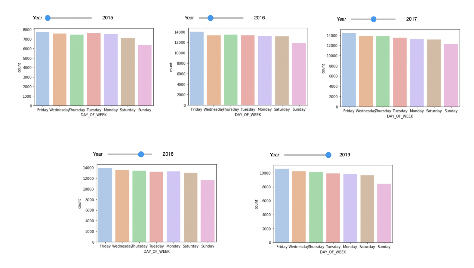png

Based on the below, the Peak Crime hour were at 12pm and between 4pm to 7pm. This trend was seen in all five years. 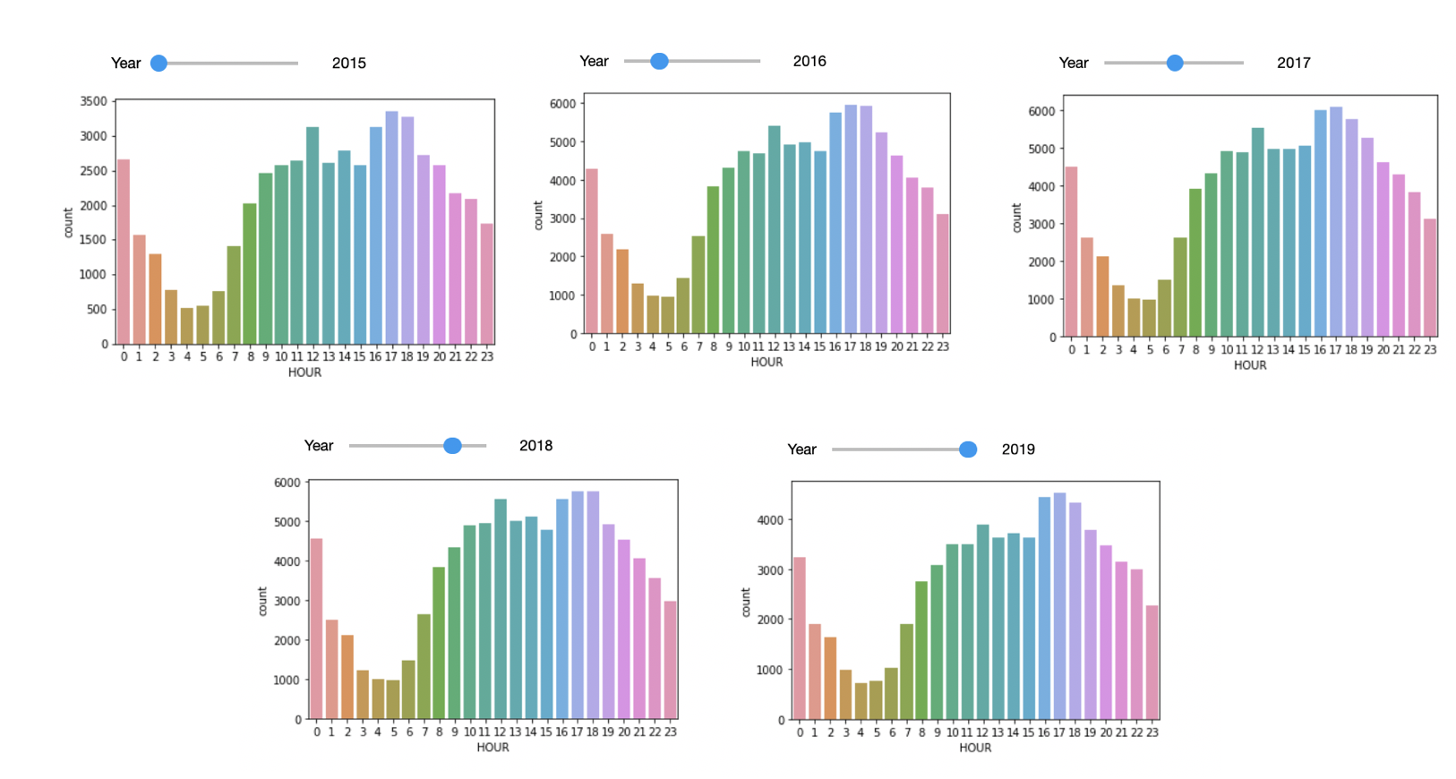png

Below graph shows the top 70% offense code group or crime type based on the number of times they occured through out the entire 5 years. This is the dependent variable that we will predict in the model. 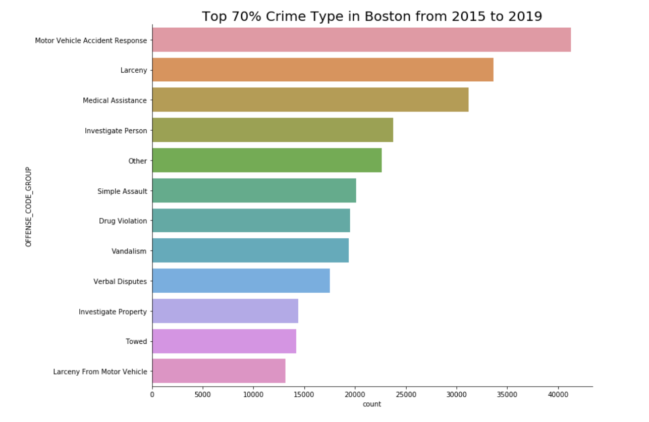png

Looking at the crime density, the northern areas seemed to have more crime than the southern Boston areas. Below graph shows the number of crime occured grouped by the district. 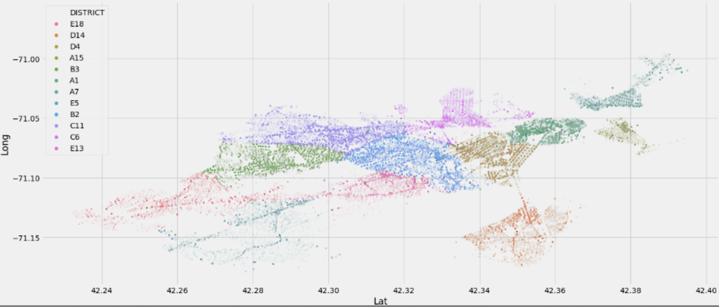png

The figures below depicts the top 70% crime offense code group or crime type. It is clearly shown that some crimes happened more often in specific areas while some other occured almost evenly all throughout Boston. 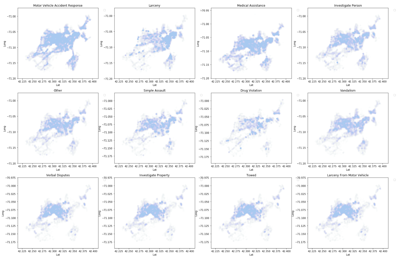png

Part 3

Building The Model

In this section I will talk about the detailed steps I took in building the prediction.

Target User Police Authority
Prediction Method Using Artificial Neural Network in Keras and Tensorflow, I will predict which type of “Offense Code Group” or Crime Type will happen in a specific location and time.
Outlier Treatment and Feature Engineering Based on the EDA result, I am removing all the observations for the bottom 30% crime incidents. This is to improve my model performance and to negate outliers. Additionally, I created 2 new variables, to group the months with season variable and to grouped the address by the top 10% highest crime addresses.
Feature Selection and Dimension Reduction Since the dataset did not have many variables to begin with, I decided to include all of the independent variables to train my first model and then conduct the backward elimination method for dimension reduction.

Top 70% Crime Offense Code Group or Crime Type

{'OFFENSE_CODE_GROUP': {'Drug Violation': 0,
  'Investigate Person': 1,
  'Investigate Property': 2,
  'Larceny': 3,
  'Larceny From Motor Vehicle': 4,
  'Medical Assistance': 5,
  'Motor Vehicle Accident Response': 6,
  'Other': 7,
  'Simple Assault': 8,
  'Towed': 9,
  'Vandalism': 10,
  'Verbal Disputes': 11}}

Correlation Matrix to Test for Collinearity

Before I started building my model, it’s always a good idea to see how the current independent variables are related to the dependent variable. A correlation matrix can also help identify collinearity between independent variables. In this case, I plotted the correlation matrix for the continuous independent variables and ran a chi-squared test for the categorical variables.

Based on the correlation test, year seemed to have very minimal correlation with the dependent variable. 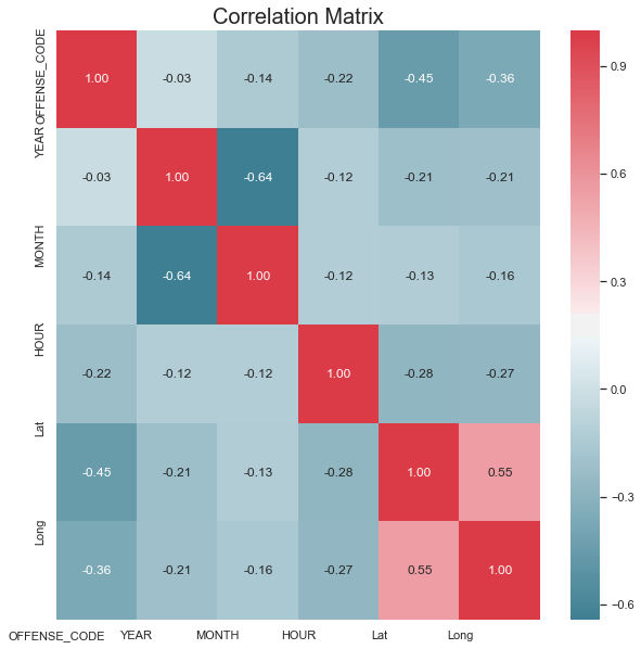png

Chi-Squared Test to Test the Significant Relationship between Independent Var vs Dependent Var

There were only 2 categorical variables in the data and they were both have significant relationship with the dependent variable. However, I decided not to use the SHOOTING(yes/no) variable as the data would only be available after the incident or the crime had happened.

SHOOTING and Offense Code Group
Chi Squared Value :
186.06374094281534
P-Value :
5.728576066226494e-34
 
Day of Week and Offense Code Group
Chi Squared Value :
1817.9993218058914
P-Value :
0.0

Preparing the Data Format for The Model

##Categorizing the season column using Dummy Vars : the reason is because there is no Hierarchy..
#meaning that, "Fall IS NOT Higher or Better than Summer"

def data_prep(df_clean):
    
    #date time split 2019-10-13 09:28:24
    def parse_time(x):
        DD=datetime.strptime(x,"%Y-%m-%d %H:%M:%S")
        time=DD.hour 
        day=DD.day
        month=DD.month
        year=DD.year
        mins=DD.minute
        return time,day,month,year,mins
    
    parsed = np.array([parse_time(x) for x in df_clean.occured_on_dttm])
    
    df_clean['Dates'] = pd.to_datetime(df_clean['occured_on_dttm'])
    df_clean['WeekOfYear'] = df_clean['Dates'].dt.weekofyear
    df_clean['Hour'] = parsed[:,[0]]
    df_clean['day'] = parsed[:,[1]]
    df_clean['month'] = parsed[:,[2]]
    df_clean['year'] = parsed[:,[3]]
    df_clean['mins'] = parsed[:,[4]]
    
    
        
    #adding season variable
    def get_season(x):
        if x in [5, 6, 7]:
            r = 'summer'
        elif x in [8, 9, 10]:
            r = 'fall'
        elif x in [11, 12, 1]:
            r = 'winter'
        elif x in [2, 3, 4]:
            r = 'spring'
        return r
    
    df_clean['season'] = [get_season(i) for i in crime.MONTH]
        
        
    #grouping street       
    streetcount = df_clean.groupby(['STREET'], as_index=False).agg({"INCIDENT_NUMBER":"count"}).sort_values(by='INCIDENT_NUMBER', ascending=False).head(8)
    streetcount['odds'] = [round(i/(len(df_clean.STREET)+1),3) for i in streetcount.INCIDENT_NUMBER]
    streetcount.drop(['INCIDENT_NUMBER'],axis=1,inplace=True)
    df_clean = pd.merge(left=df_clean,right=streetcount,how='left',left_on='STREET',right_on='STREET')
    
    
    #dummy variables
    df_clean_onehot = pd.get_dummies(df_clean, columns=['season'], prefix = [''])
    s = (len(list(df_clean_onehot.columns))-len(df_clean.season.value_counts()))
    df_clean = pd.concat([df_clean,df_clean_onehot.iloc[:,s:]], axis=1)

    ##Categorizing the DayOFWeek column using Dummy Vars 
    df_clean_onehot = pd.get_dummies(df_clean, columns=['DAY_OF_WEEK'], prefix = [''])
    l = (len(list(df_clean_onehot.columns))-len(df_clean.DAY_OF_WEEK.value_counts()))
    df_clean = pd.concat([df_clean,df_clean_onehot.iloc[:,l:]],axis=1)

    ##Categorizing the MONTH column using Dummy Vars : the reason is because there is no Hierarchy..
    #meaning that, "FEB IS NOT Higher or Better than JAN"
    #This insight was shown from the EDA result (forecasting data with trend might be a different case)

    df_clean_onehot = pd.get_dummies(df_clean, columns=['month'], prefix = ['month'])
    n = (len(list(df_clean_onehot.columns))-len(df_clean.MONTH.value_counts()))
    df_clean = pd.concat([df_clean,df_clean_onehot.iloc[:,n:]],axis=1)

    ##Categorizing the District column using Dummy Vars 

    df_clean_onehot = pd.get_dummies(df_clean, columns=['DISTRICT'], prefix = [''])
    o = (len(list(df_clean_onehot.columns))-len(df_clean.DISTRICT.value_counts()))
    df_clean = pd.concat([df_clean,df_clean_onehot.iloc[:,o:]],axis=1)

    ##changing the Output Variables to integer
    labels = df_clean['OFFENSE_CODE_GROUP'].astype('category').cat.categories.tolist()
    replace_with_int = {'OFFENSE_CODE_GROUP' : {k: v for k,v in zip(labels,list(range(0,len(labels))))}}
    df_clean.replace(replace_with_int, inplace=True)

    #Normalizing the columns
    def norm_func(i):
        r = (i-min(i))/(max(i)-min(i))
        return(r)

    df_clean['normHour']=norm_func(df_clean.HOUR)
    df_clean['normmins']=norm_func(df_clean.mins)
    df_clean['normdate_day']=norm_func(df_clean.day)
    df_clean['normLat']=norm_func(df_clean.Lat)
    df_clean['normLong']=norm_func(df_clean.Long)
    df_clean['normmonth']=norm_func(df_clean.month)
    df_clean['normyear']=norm_func(df_clean.year)
    df_clean['normWeekOfYear']=norm_func(df_clean.WeekOfYear)



    ##removing the unused columns
    df_clean.drop(columns = [ 'Unnamed: 0', 'INCIDENT_NUMBER', 'OFFENSE_CODE',
       'OFFENSE_DESCRIPTION', 'DISTRICT', 'REPORTING_AREA', 'SHOOTING', 'YEAR',
       'MONTH', 'DAY_OF_WEEK', 'HOUR', 'UCR_PART', 'STREET', 'Lat', 'Long',
       'Location_lat', 'Location_long', 'date_occured', 'occured_on_dttm','Dates',
        'WeekOfYear','Hour','day','month','year','mins','season'], axis = 1,inplace=True)
    return(df_clean)

Splitting the Train & Test Data for Model

Using the holdout method, I randomly split the dataset into 80% for training, and 20% for testing.

split = np.random.rand(len(crime_clean)) < 0.8
train = crime_clean[split]
test = crime_clean[~split]

print('entire dataset :',len(crime_clean.OFFENSE_CODE_GROUP.value_counts().index), 'offense codes')
print('train dataset :',len(crime_clean.OFFENSE_CODE_GROUP.value_counts().index), 'offense codes')
print('test dataset :',len(crime_clean.OFFENSE_CODE_GROUP.value_counts().index), 'offense codes')

entire dataset : 12 offense codes
train dataset : 12 offense codes
test dataset : 12 offense codes

Below shows the format in which I will fit the data into my model.

train1.info()

<class 'pandas.core.frame.DataFrame'>
RangeIndex: 217154 entries, 0 to 217153
Data columns (total 43 columns):
OFFENSE_CODE_GROUP    217154 non-null int64
_fall                 217154 non-null uint8
_spring               217154 non-null uint8
_summer               217154 non-null uint8
_winter               217154 non-null uint8
_Friday               217154 non-null uint8
_Monday               217154 non-null uint8
_Saturday             217154 non-null uint8
_Sunday               217154 non-null uint8
_Thursday             217154 non-null uint8
_Tuesday              217154 non-null uint8
_Wednesday            217154 non-null uint8
month_1               217154 non-null uint8
month_2               217154 non-null uint8
month_3               217154 non-null uint8
month_4               217154 non-null uint8
month_5               217154 non-null uint8
month_6               217154 non-null uint8
month_7               217154 non-null uint8
month_8               217154 non-null uint8
month_9               217154 non-null uint8
month_10              217154 non-null uint8
month_11              217154 non-null uint8
month_12              217154 non-null uint8
_A1                   217154 non-null uint8
_A15                  217154 non-null uint8
_A7                   217154 non-null uint8
_B2                   217154 non-null uint8
_B3                   217154 non-null uint8
_C11                  217154 non-null uint8
_C6                   217154 non-null uint8
_D14                  217154 non-null uint8
_D4                   217154 non-null uint8
_E13                  217154 non-null uint8
_E18                  217154 non-null uint8
_E5                   217154 non-null uint8
normHour              217154 non-null float64
normmins              217154 non-null float64
normdate_day          217154 non-null float64
normLat               217154 non-null float64
normLong              217154 non-null float64
normmonth             217154 non-null float64
normWeekOfYear        217154 non-null float64
dtypes: float64(7), int64(1), uint8(35)
memory usage: 20.5 MB

Training the neural network model

Model 1 - Used all variables, 1 layer, 20 epoch

from sklearn.metrics import roc_auc_score

model = Sequential()
model.add(Dense(12, input_shape=(47,)))
#model.add(Dense(128, activation='relu', input_dim=512))
model.add(Dense(90, activation='relu', input_dim=128))
model.add(Dense(12, activation='softmax', input_dim=90))
model.compile(loss='sparse_categorical_crossentropy', metrics=['accuracy']
              , optimizer='adam')

# The fit() method - trains the model
model.fit(TrainData, TrainLabels, nb_epoch=20)

/Library/Frameworks/Python.framework/Versions/3.7/lib/python3.7/site-packages/ipykernel_launcher.py:11: UserWarning: The `nb_epoch` argument in `fit` has been renamed `epochs`.
  # This is added back by InteractiveShellApp.init_path()


Epoch 1/20
216985/216985 [==============================] - 7s 34us/step - loss: 2.3499 - accuracy: 0.1841
Epoch 2/20
216985/216985 [==============================] - 6s 30us/step - loss: 2.3141 - accuracy: 0.1961 0s
Epoch 3/20
216985/216985 [==============================] - 6s 28us/step - loss: 2.2980 - accuracy: 0.2019 1s - loss: 2.2989 - accura - E
Epoch 4/20
216985/216985 [==============================] - 7s 33us/step - loss: 2.2897 - accuracy: 0.2049
Epoch 5/20
216985/216985 [==============================] - 7s 30us/step - loss: 2.2855 - accuracy: 0.2058
Epoch 6/20
216985/216985 [==============================] - 7s 31us/step - loss: 2.2820 - accuracy: 0.2076
Epoch 7/20
216985/216985 [==============================] - 7s 30us/step - loss: 2.2798 - accuracy: 0.2080
Epoch 8/20
216985/216985 [==============================] - 6s 30us/step - loss: 2.2774 - accuracy: 0.2090
Epoch 9/20
216985/216985 [==============================] - 7s 30us/step - loss: 2.2760 - accuracy: 0.2093
Epoch 10/20
216985/216985 [==============================] - 6s 28us/step - loss: 2.2746 - accuracy: 0.2100
Epoch 11/20
216985/216985 [==============================] - 6s 30us/step - loss: 2.2731 - accuracy: 0.2102
Epoch 12/20
216985/216985 [==============================] - 7s 32us/step - loss: 2.2715 - accuracy: 0.2114
Epoch 13/20
216985/216985 [==============================] - 6s 28us/step - loss: 2.2700 - accuracy: 0.2111 0s - l
Epoch 14/20
216985/216985 [==============================] - 7s 31us/step - loss: 2.2688 - accuracy: 0.2129
Epoch 15/20
216985/216985 [==============================] - 7s 32us/step - loss: 2.2672 - accuracy: 0.2132
Epoch 16/20
216985/216985 [==============================] - 6s 29us/step - loss: 2.2660 - accuracy: 0.2142
Epoch 17/20
216985/216985 [==============================] - 7s 30us/step - loss: 2.2644 - accuracy: 0.2151
Epoch 18/20
216985/216985 [==============================] - 6s 30us/step - loss: 2.2630 - accuracy: 0.2154
Epoch 19/20
216985/216985 [==============================] - 6s 30us/step - loss: 2.2611 - accuracy: 0.2157
Epoch 20/20
216985/216985 [==============================] - 6s 29us/step - loss: 2.2597 - accuracy: 0.2167 0s - l





<keras.callbacks.callbacks.History at 0x13bf28c90>

Evaluate the model on the cleaned test data

54638/54638 [==============================] - 1s 14us/step
Test Loss:
2.2633479155106166
Test Accuracy:
0.21847432851791382

Model 2 - Dropped street grouping and year variables, 2 layers, 20 epoch

model1 = Sequential()
model1.add(Dense(12, input_shape=(42,)))
model1.add(Dense(128, activation='relu', input_dim=512))
model1.add(Dense(90, activation='relu', input_dim=128))
model1.add(Dense(12, activation='softmax', input_dim=90))
model1.compile(loss='sparse_categorical_crossentropy', metrics=['accuracy']
               , optimizer='adam')

# The fit() method - trains the model
model1.fit(Train1Data, Train1Labels, nb_epoch=20)

/Library/Frameworks/Python.framework/Versions/3.7/lib/python3.7/site-packages/ipykernel_launcher.py:10: UserWarning: The `nb_epoch` argument in `fit` has been renamed `epochs`.
  # Remove the CWD from sys.path while we load stuff.


Epoch 1/20
217154/217154 [==============================] - 8s 36us/step - loss: 2.3550 - accuracy: 0.1838
Epoch 2/20
217154/217154 [==============================] - 9s 40us/step - loss: 2.3194 - accuracy: 0.1915
Epoch 3/20
217154/217154 [==============================] - 8s 37us/step - loss: 2.3096 - accuracy: 0.1955 1s - loss: 2.3098  - ETA: 0s - loss: 2.3096 -  - ETA: 0s - loss: 2.309
Epoch 4/20
217154/217154 [==============================] - 8s 35us/step - loss: 2.3029 - accuracy: 0.1981
Epoch 5/20
217154/217154 [==============================] - 8s 38us/step - loss: 2.2967 - accuracy: 0.2014E
Epoch 6/20
217154/217154 [==============================] - 8s 36us/step - loss: 2.2916 - accuracy: 0.2031
Epoch 7/20
217154/217154 [==============================] - 9s 40us/step - loss: 2.2867 - accuracy: 0.2061
Epoch 8/20
217154/217154 [==============================] - 9s 39us/step - loss: 2.2818 - accuracy: 0.2090
Epoch 9/20
217154/217154 [==============================] - 8s 35us/step - loss: 2.2770 - accuracy: 0.2112
Epoch 10/20
217154/217154 [==============================] - 7s 33us/step - loss: 2.2732 - accuracy: 0.2128
Epoch 11/20
217154/217154 [==============================] - 7s 33us/step - loss: 2.2688 - accuracy: 0.2147
Epoch 12/20
217154/217154 [==============================] - 7s 33us/step - loss: 2.2652 - accuracy: 0.2154 5s - loss: 2.2637 - accuracy - E - ETA: 0s - loss: 2.2655 - accuracy:  - ETA: 0s - loss: 2.2655 - accu - ETA: 0s - loss: 2.2654 - accu
Epoch 13/20
217154/217154 [==============================] - 8s 37us/step - loss: 2.2612 - accuracy: 0.2178
Epoch 14/20
217154/217154 [==============================] - 8s 37us/step - loss: 2.2572 - accuracy: 0.2197
Epoch 15/20
217154/217154 [==============================] - 8s 35us/step - loss: 2.2540 - accuracy: 0.2207
Epoch 16/20
217154/217154 [==============================] - 8s 38us/step - loss: 2.2501 - accuracy: 0.2223
Epoch 17/20
217154/217154 [==============================] - 7s 34us/step - loss: 2.2466 - accuracy: 0.2238
Epoch 18/20
217154/217154 [==============================] - 7s 34us/step - loss: 2.2437 - accuracy: 0.2245 0s - los
Epoch 19/20
217154/217154 [==============================] - 7s 33us/step - loss: 2.2407 - accuracy: 0.2259
Epoch 20/20
217154/217154 [==============================] - 7s 34us/step - loss: 2.2386 - accuracy: 0.2265 0s - loss: 2.2389 - accura





<keras.callbacks.callbacks.History at 0x14549a650>

Evaluating on Test Data

54469/54469 [==============================] - 1s 15us/step
Test Loss:
2.2557787604998083
Test Accuracy:
0.22216306626796722

Part 4

Model Comparison and Conclusion

The baseline probability was ~8.3% for each class since there were 12 classes in the dependent variable. In the first model, I fitted all the independent variables into the model which resulted in an accuracy of ~21.8% and a loss of ~2.26. This is considerably good since this was a multiclass classification with 12 classes.

However, there were definitely room for improvements in the model performance. In the second model, I decided to remove the year variable based on the correlation test result and the address grouping variable to enhance the performance of the model. The result was that the accuracy slightly improved to ~22.2% and the loss was reduced slightly.

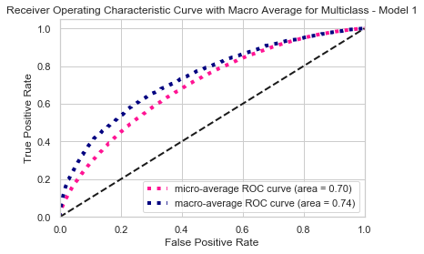
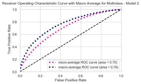
Though the average TPR and FPR comparison in the ROC curve showed that model 2 has bigger area under the curve compared to model 1, this performance assessment in inaccurate for non-binary classification model. Therefore, I would rely more the loss and accuracy to measure the model performance.

Based on the above, I chose model 2 to predict the crime type or offense code in Boston.

ROC Curve

MODEL 1

png

MODEL 2

png

Model Raw Output

predictions = model1.predict_proba(Test1Data)
predictiondata=pd.DataFrame(data=predictions) 
predictiondata.drop([0], axis =1, inplace = True) #removing the 0th class auto created by TF
predictiondata.rename(columns = {i:j for i,j in zip(predictiondata.columns,labels)}, inplace = True)
predictiondata['MaxProb'] = [np.max(i) for i in predictions]
predictiondata['MaxProbLabel'] = [labels[np.argmax(i)] for i in predictions]

	Drug Violation	Investigate Person	Investigate Property	Larceny	Larceny From Motor Vehicle	Medical Assistance	Motor Vehicle Accident Response	Other	Simple Assault	Towed	Vandalism	MaxProb	MaxProbLabel
9860	0.010175	0.000684	0.964066	0.005465	0.003356	0.008226	0.002629	0.002399	0.000011	0.001224	0.000005	0.964066	Larceny
13580	0.033826	0.004403	0.001145	0.000043	0.024009	0.001463	0.001869	0.000129	0.000039	0.000456	0.000544	0.932073	Drug Violation
37795	0.026715	0.001182	0.908468	0.008588	0.009570	0.019438	0.008087	0.008032	0.000114	0.002578	0.000042	0.908468	Larceny
24645	0.024893	0.001246	0.901784	0.012499	0.007624	0.018414	0.006875	0.011354	0.000050	0.004500	0.000047	0.901784	Larceny
26403	0.050741	0.015595	0.002573	0.000145	0.033954	0.004519	0.005075	0.000466	0.000145	0.000760	0.001430	0.884597	Drug Violation

</div>

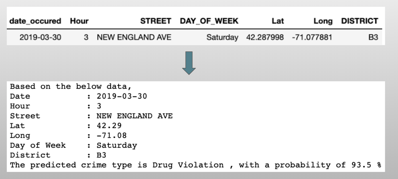
Final Prediction Output

png

Analysis and Report Written by : Jennifer Siwu