In this project, I worked with a group of 5 for our last final project in my Master’s degree. With this, we aimed to understand customer complaints on social media, specifically Twitter, regarding the major airlines in the US. To learn more about our project and the codes we used to implement it, please check out our github repository here. This article was also featured by AnalyticsVidhya on Medium.com.

Objective

Customer sentiment:
To identify positive and negative opinions, emotions, and evaluations.
Identify negative topics:
Derive negative topics that people are likely to mention when talking with their experience with airlines.
Derive actionable insights:
Insights may later be used by airlines in planning and execution of customer service initiatives, media relationships etc.

Dataset

The data originally came from Crowdflower’s Data for Everyone library, which was then made available to us on Kaggle. The twitter data was scraped from February 2015 for 2 weeks. It contains over 14K tweets and their sentiment (positive, neutral, or negative) regarding 6 major airlines in the US.

Data Analysis

Before jumping into modeling, we did some preliminary data analysis to understand some patterns or trends in the data.

Twitter mood distribution & Tweet counts by airline: The tweets data has 63% of negative, 16% positive and 21% neutral tweets. United airlines has the most #tweets followed by US airways, American and Southwest airlines.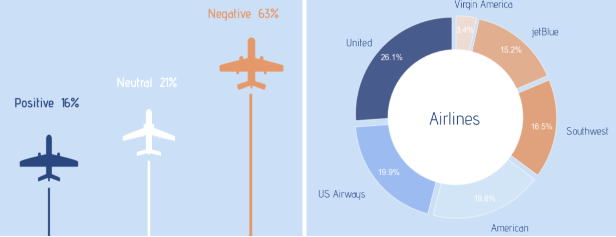

Tweet sentiment by Location: Most of the tweets were concentrated around the east coast. This is due to the busiest international airports being around that.

Twitter mood by airline: American, United and US airways have >60% negative tweets and have a lot of negative retweets.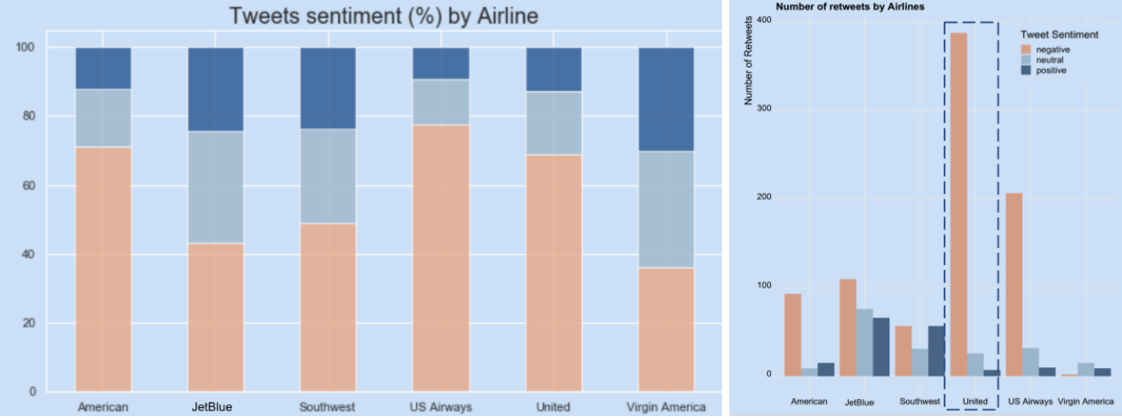

The Distribution of Word Count between Sentiment: Based on the below density curve and boxplot, we can see that negative tweets are generally wordier than the other sentiments. Our One-way Anova Test concluded that there are indeed differences in word count between these sentiments (p < 0.01).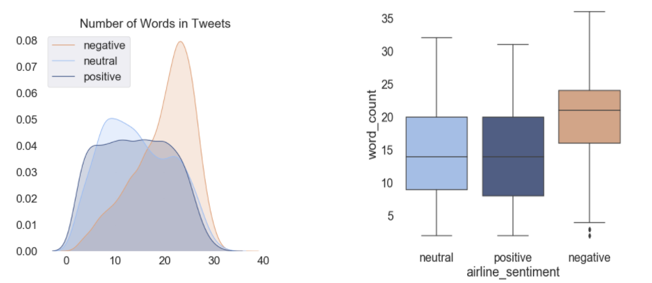

Top words for negative tweets: The word cloud for negative tweets indicates high frequency words such as delayed, hold, bag, hour, call.

Approach

Approach 1 – Sentiment Analysis

Method

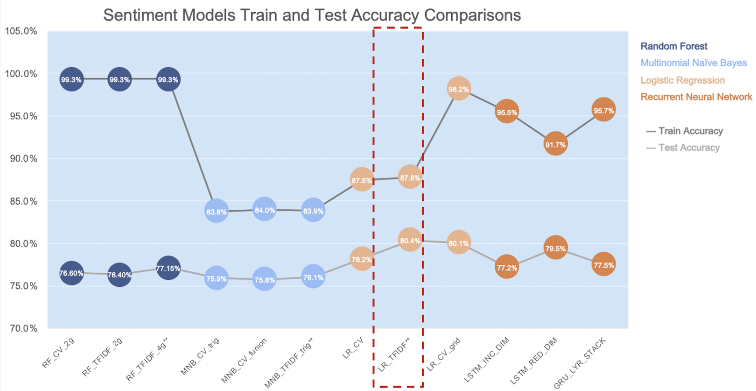(**) Indicates Best Model in each algorithm

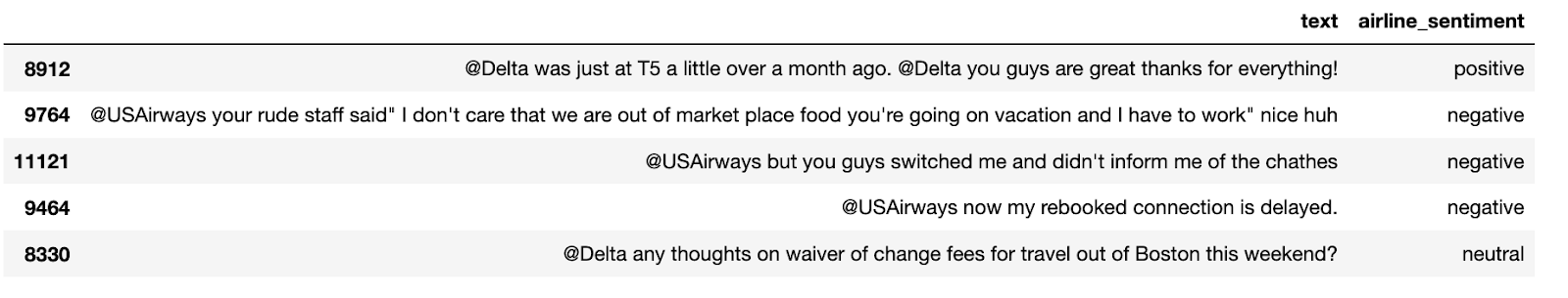
Based on the model result summary shown above, we chose the Logistic Regression with TFIDF as our best model to predict the sentiment. Below, we will talk about our approach for this model. Since we are only interested in the content of the tweet and sentiment level of each tweet, we extracted the corresponding two columns, which are ‘text’ and ‘airline_sentiment’. The screenshot below shows 5 random samples of texts and their sentiment levels.

1.Text Processing
First off, we cleaned the text using regular expressions to remove hashtags, symbols, mentions, URLs, digits, and punctuations. After applying previous steps, texts had some extra white spaces that later the tokenizer can split as words. That said, we removed those extra spaces. In addition, we ensured to remove all single characters, for example, “ it’s ” can be transformed to “ it s “, then we need to remove “s” since it doesn’t have any meaning. For stemming, we noticed that although Porter is the most commonly used stemmer, also one of the most gentle stemmers, there are many words we missed their original meaning after taking stemming and ended up lowering the accuracy. Therefore, we decided to not add stemming for the text cleansing part.

Also, we set up stopwords and excluded some words that indicated negativity such as “not”, “no” as well as updated some words that are not meaningful to predict the sentiment.

Next up, in order to segment text into words, we did tokenization and below shows the examples.

def clean_text(txt):
    
    """
    removing all hashtags , punctuations, stop_words  and links, also stemming words 
    """
    txt = txt.lower()
    def remove_stopwords(txt):
        return [t for t in txt if t not in stop]
    #txt = re.sub(r"(?<=\w)nt", "not",txt) #change don't to do not cna't to cannot 
    txt = re.sub(r"(@\S+)", "", txt)  # remove hashtags
    txt = re.sub(r'\W', ' ', str(txt)) # remove all special characters including apastrophie 
    txt = txt.translate(str.maketrans('', '', string.punctuation)) # remove punctuations 
    txt = re.sub(r'\s+[a-zA-Z]\s+', ' ', txt)   # remove all single characters (it's -> it s then we need to remove s)
    txt = re.sub(r'\s+', ' ', txt, flags=re.I) # Substituting multiple spaces with single space
    txt = re.sub(r"(http\S+|http)", "", txt) # remove links 
#    txt = ' '.join([PorterStemmer().stem(word=word) for word in txt.split(" ") if word not in stop_words ]) # stem & remove stop words
    txt = ''.join([i for i in txt if not i.isdigit()]).strip() # remove digits ()
    return txt
df['cleaned_text'] = df['text'].apply(clean_text)
re_tok = re.compile(f'([{string.punctuation}""¨«»®´·º½¾¿¡§£₤''])')
def tokenize(s): 
    return re_tok.sub(r' \1 ', s).split()
df['tokenized'] = df['cleaned_text'].apply(lambda row: tokenize(row))
stop = set(stopwords.words('english'))
stop.update(['amp', 'rt', 'cc'])
stop = stop - set(['no', 'not'])
def remove_stopwords(row):
    return [t for t in row if t not in stop]
df['tokenized'] = df['tokenized'].apply(lambda row: remove_stopwords(row))

df[['text', 'tokenized']].head()

2.Text vectorization
Then we did the text vectorization to transform documents into vectors using CountVectorizer and TFIDF.

*TFIDF : The hyperparameter without using grid search, we used maximum features with 2500, and ignored terms that have a document frequency strictly higher than 0.8, and lower than 7. For the solver we used newton-cg since it’s robust to unscaled dataset and performs better with multinomials with an l2 penalty, which is also known as Ridge. Ridge includes all variables in the model, though some are shrunk as well as it is less computationally intensive than the lasso. We chose 10 for the Inverse of regularization strength.

*Countvectorizer : The hyper parameter without using grid search, we ignored terms that have a document frequency strictly lower than 5 and had unigram and bigram for n gram ranges.

*CV Gridsearch : Then we tried with hyper parameters recommended by gridsearch which are:
*C: 3
*Penalty: ‘l2’
*max_df: 0.5 (ignores terms that appear in more than 50% of the documents)
*min_df: 1 (ignore terms that appear in less than 1 documents)
*ngram_range: (1, 2)

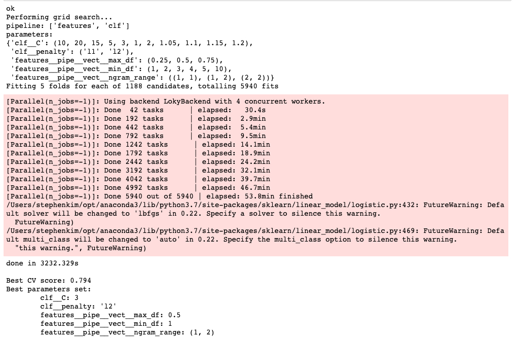
However, the accuracy turns out to be lower than the previous two models. When looking at parameters we noticed that the hyper parameters recommended by gridsearch are more strict in terms of dropping the terms. For example, TFIDF ignores terms that appear in less than 7 documents whereas gridsearch suggests ignoring terms that appear in less than 1 document (min_df).

Result
Among those 3 models, logistic regression using TFIDF had the highest test accuracy at 80.3%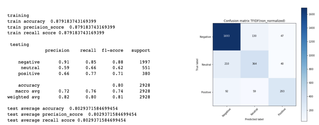

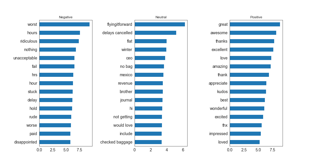
With logistic regression classifiers, we were able to plot the most important coefficients that are considered to make the predictions for each sentiment level. As you can see below, for negative, “worst”, “hours”, “ridiculous” or words specifically related to hours appear to highly contribute to the prediction. And similarly, for positive, “great”, “awesome”, “thanks” and words related to gratitude highly contribute to the sentiment prediction.

learning & challenges

We believe one of the reasons TFIDF performed better than countvectorizer is that it can be more useful in capturing frequent yet not meaningful words since it weighs down those words such as “LOL” or “ASAP” while it scales up the unique words related to customer experience. One of challenges of performing sentiment analysis on Twitter is that since each of Twitteruser speaks differently about their experience, there are many slangs, new words, acronym, abbreviation, curse, or simply misspelled words that can hard to capture with current text cleaning packages or regex especially when data is large. For the next step, we would like to search for better text cleaning packages that can reduce issues mentioned above.

Approach 2 – Topic Modeling with LDA

With approach 1, we were able to identify the sentiment of tweets with a relatively high degree of accuracy. To take the analysis a step further, we wanted to understand what are the general topics or categories that people are raising their concern about on the negative tweets. One of the most popular and well adopted algorithms for topic modeling is the LDA (Latent Dirichlet Allocation).

Latent Dirichlet Allocation (LDA) The way that LDA works is that it assumes each document consists of a mix with various topics and every topic consists of a mix with various words. It builds a topic per document model and words per topic model, which are based upon Dirichlet distributions. The below graph helps explain the algorithm flow.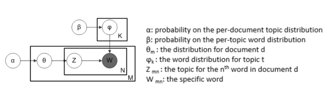

Using our data, we can build a dictionary to train the LDA model. Then, the LDA model will output the top words within each topic, from which the analyst then can categorize them into topic names (yes, it does require that manual part but, it still works well).

Method

1.Text Preprocessing
First and most important step in LDA is data cleaning or, more specifically, stopwords removal. This is also considered as the major drawback of LDA modeling as we need to clean and nitpick a lot of words which don’t really indicate topics. For example, in this context, words such as “baggage” and “delay” indicate different topics or complaint categories. However, words such as “completely” or “chicago” do not.

The steps we took in text preprocessing were (As shown in the code below):
      1. Regex: Removing Flight Number, Emoji, Hashtags, Twitter Username, Text Punctuations, and Symbols
      2. Html Parser + Lowercase
      3. Stopwords Extension (>500 words), including:
         -US city names
         -Airline Names
         -Date, Time, Day of Week
         -Spacy Tokens
         -Remove Adjective and Conjunction
         -Stemmer + Lemmatizer

cities = pd.read_csv("https://raw.githubusercontent.com/grammakov/USA-cities-and-states/master/us_cities_states_counties.csv",sep="|")
cities = cities.iloc[:,:2]
cities.drop_duplicates(keep='first',inplace=True)
#preprocess data
def preprocess(text):
    stopwords = set(STOPWORDS)
    stopwords.update(exclude_word_list) 
#this list was saved to csv and made available on our Github repo
#stopwords.update([i for i in ts])
    # stopwords.update([str(i).lower() for i in cities.City]) #removing City names in US
    r = re.compile(r'(?<=\@)(\w+)') #remove words after tags --> usually twitter account
    ra = re.compile(r'(?<=\#)(\w+)') #remove words after hashtags
    ro = re.compile(r'(flt\d*)') #remove words after flight number
    names = r.findall(text.lower())
    hashtag = ra.findall(text.lower())
    flight = ro.findall(text.lower())
    lmtzr = WordNetLemmatizer()
    def stem_tokens(tokens, lemmatize):
        lemmatized = []
        for item in tokens:
            lemmatized.append(lmtzr.lemmatize(item,'v'))
        return lemmatized
    def deEmojify(inputString):
        return inputString.encode('ascii', 'ignore').decode('ascii')
    
    doc = nlp(text)
    text = deEmojify(text)
    soup = BeautifulSoup(text)
    text = soup.get_text()
    text = "".join([ch.lower() for ch in text if ch not in string.punctuation])
    tokens = nltk.word_tokenize(text)
    tokens = [ch for ch in tokens if len(ch)>4] #remove words with character length below 2
    tokens = [ch for ch in tokens if len(ch)<=15] #remove words with character length above 15 
    lemm = stem_tokens(tokens, lmtzr)
    lemstop = [i for i in lemm if i not in stopwords]
    lemstopcl = [i for i in lemstop if i not in names]
    lemstopcl = [i for i in lemstopcl if i not in hashtag]
    lemstopcl = [i for i in lemstopcl if i not in flight]
    lemstopcl = [i for i in lemstopcl if not i.isdigit()]
    lemstopcl1 = [i for i in lemstopcl if i not in t]
    return lemstopcl

2.Choosing the Number of Topics (K)
Once we’ve preprocessed the words into tokens, we can create a dictionary (or bag of word) that contains the number of times a word appears in the training dataset. Using this bag of words, we can then train our LDA model.

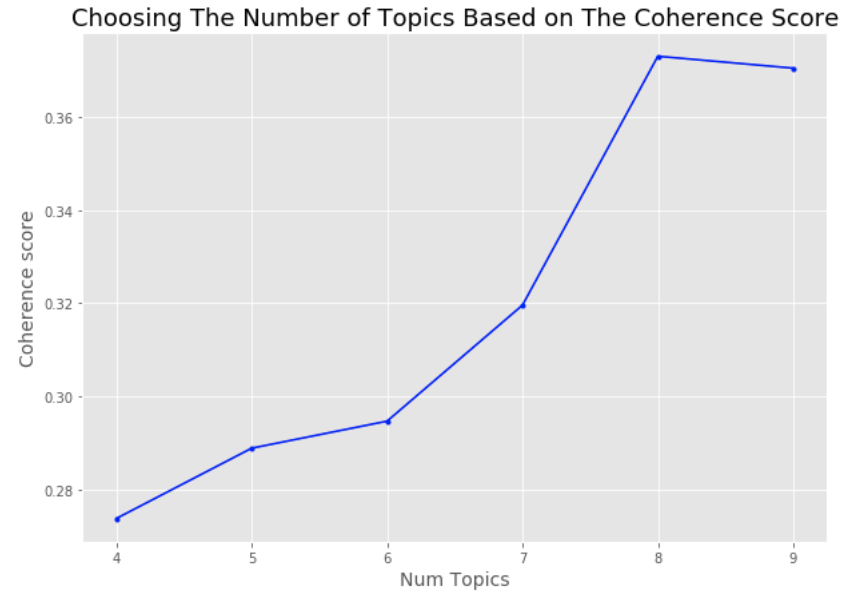
We also need to identify the number of topics (K) for LDA (similar to identifying the k for k-means clustering). Although there are many ways to identify the optimal number of topics, the most adopted ones are using the perplexity score and coherence score. The idea is the less the perplexity score and the higher the coherence score, the better that “K” is. (click here if you would like to learn more about coherence or perplexity score). Based on the plot below, we identified that the best “K” for this data is 8. Therefore, we used that to train our LDA model.

def compute_coherence_values(dictionary, corpus, texts, start, stop):
    """
    Compute c_v coherence for various number of topics
    """
    coherence_values = []
    model_list = []
    for num_topics in range(start, stop):
        model = gensim.models.ldamodel.LdaModel(corpus=corpus, 
                                              num_topics=num_topics,
                                              id2word=id2word,
                                              random_state=90,
                                              alpha='auto',
                                              eta='auto',
                                              per_word_topics=True)
        model_list.append(model)
        coherencemodel = CoherenceModel(model=model, texts=texts,
                             dictionary=dictionary, coherence='c_v')
        coherence_values.append(coherencemodel.get_coherence())
    return model_list, coherence_values
start=4
stop=9
model_list, coherence_values = compute_coherence_values(dictionary=id2word, 
                                    corpus=corpus,
                                    texts=processed_docs,
                                    start=start, stop=stop)

3.Training the LDA model
Using k of 8, we received a perplexity score of -9.34 and coherence score of 0.60, which is pretty decent considering there are more than 5 topics.

%%time
# Create Dictionary
id2word = gensim.corpora.Dictionary(processed_docs)
# Create Corpus: Term Document Frequency
corpus = [id2word.doc2bow(text) for text in processed_docs]
# Build LDA model
lda_model1 = gensim.models.ldamodel.LdaModel(corpus=corpus,
                                           id2word=id2word,
                                           num_topics=8, 
                                           random_state=123,
                                           update_every=1,
                                           chunksize=10,
                                           passes=10,
                                           alpha='auto',
                                           eta='auto',
                                           iterations=125,
                                           per_word_topics=True)
doc_lda = lda_model1[corpus]

Result
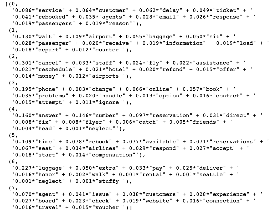
We can now print the top words within each topic to identify the topic name.

from pprint import pprint
pprint(lda_model4.print_topics())

To visualize it better, we used pyLDAvis from gensim package that outputs an interactive result of our LDA model into an html as below where each bubble represents a topic. An ideal LDA model is one where all the bubbles are separated from each other. In this case, our model is pretty good since the big bubbles (bubbles consisting more tokens in the documents) are far apart from each other with only small ones being so close to each other.

When we click on each bubble, we can see the % of tokens they include as well as the words in it with its corresponding probability score (that is the probability of that word belonging to that topic).

import pyLDAvis
from pyLDAvis import gensim
pyLDAvis.enable_notebook()
vis = pyLDAvis.gensim.prepare(lda_model4, corpus, id2word,sort_topics=False)
pyLDAvis.save_html(vis, 'ldaviz.html') #run this to save your vis as html file
vis

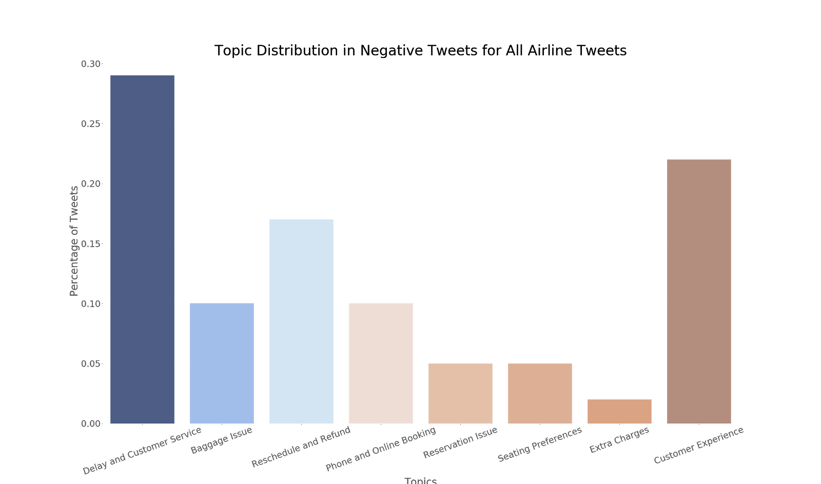
Based on the above word distributions, we decided the name the topics as below:
      Topic 1 –> Delay and Customer Service
      Topic 2 –> Baggage Issue
      Topic 3 –> Reschedule and Refund
      Topic 4 –> Phone and Online Booking
      Topic 5 –> Reservation Issue
      Topic 6 –> Seating Preferences
      Topic 7 –> Extra Charges
      Topic 8 –> Customer Experience
To make the result more interactive, we also created a short demo within a localhost site using jupyter notebook, ipywidgets, and Voila. Below are the snippets.

When we tie the LDA model results back to the business questions, we found that the top negative tweet topics are around Delays, Customer Experience, Refund/Reschedule, and Baggage. Similar to our preliminary findings on wordcloud.

Furthermore, there seems to be different topic distributions in negative tweets per airline. Take United vs American Airlines for example. United seems to have more complaints regarding baggage issues as compared to American Airlines.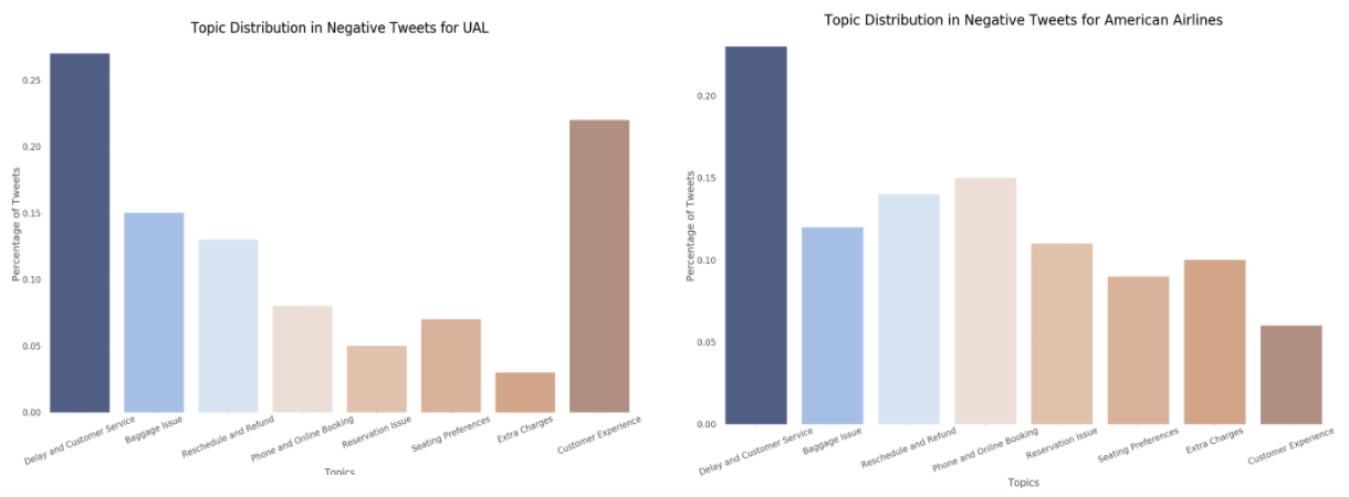

Learning and Challenges
Overall, the LDA model is a powerful and easy to use algorithm for topic analysis as the implementation time is relatively fast. However, it still requires and relies on manual work such as thoroughly removing the stopwords and correctly labeling the topics based on the top words. With that said, it requires a high attention to detail and a subject matter expert to identify which words to include/remove.

Business Implications and Recommendation

The Airline industry is a very traditional industry, with some airline general business practices that span back to their inception (1931 in the case of United Airlines). Customer feedback and sentiment was not something that the airlines always tried to gauge. J.D. Power kick-started a rush of surveys to collect consumer feedback in 1968, and it was quite a few more years until airlines had a reliable source of information to measure customer feedback information.

To gauge the validity of our findings from analyzing sentiment and topic for tweets regarding the six airlines in our scope, we compared some of our findings to facts pulled from the US Department of Transportation’s (DOT) Air Traffic Consumer Reports (ATCR). This is a report published monthly that contains various statistics regarding delays, service complaints, and other airline-related data points that compare the various US flying airlines. Statistics are also occasionally summarized to produce quarterly and annual figures.

A few fun facts:
There was an increase of 29.8% in the annual count of complaints overall for 2015
Cancellation rate for all scheduled US domestic flights was 1.5%
United Airlines ranking out of 17 airlines:
      Fewest mishandled bags: 11th
      On-time performance: 15th
      Fewest cancellations: 16th
      Fewest complaints per passenger flown: 17th

As shown above, the volume of complaints increased in 2015, and has continued to increase as the industry grows. Also, the cancellation rate may sound small at 1.5%. But when looking at a market with 9.5 million scheduled domestic flights per year, this means roughly 142,500 flights-worth of passengers are affected throughout the year. Airlines need a method to understand consumer sentiment in a more real-time method than a monthly/quarterly/annual report. It is simply not frequent enough if airlines want to be truly agile and cater to customers’ needs when they arise.

A few interesting rankings in regards to United Airlines performance were that they rank close to last place out of the US domestic airlines in on-time performance, fewest cancellations, fewest complaints, and fewest mishandled bags. From our tweets data, we saw that consumers were also complaining the most about United Airlines and for these same categories. At a high level, this shows that there is some correlation in the relationship between the twitter sentiment and topic analysis outcome with the data compiled with the ATCR, but not necessarily the causation.

(Plus, in 2015 the largest airline by passenger count was American Airlines who had fewer negative tweets than United Airlines…)

Airlines should definitely adopt some social media and sentiment/topic analysis strategy if they haven’t already done so.

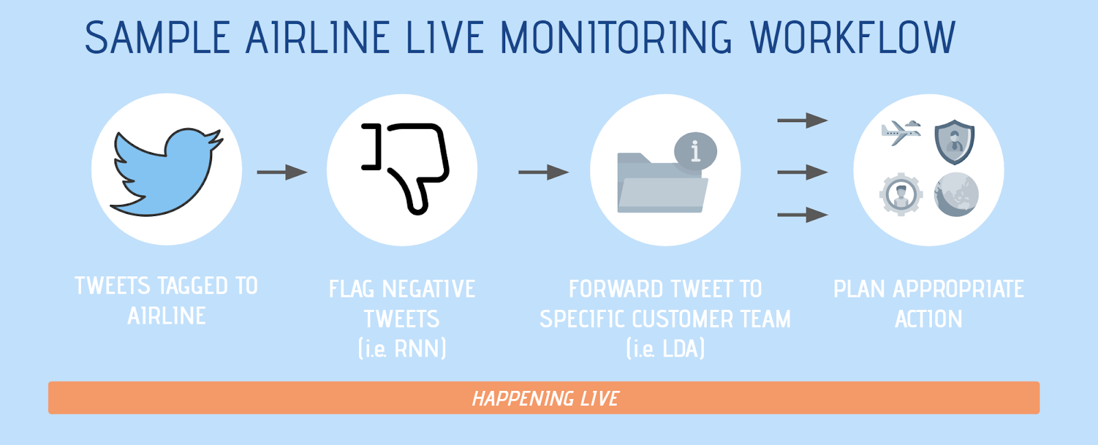
Using our 2015 Twitter data, we have observed that there is indeed some observable relationship between our analysis insights and the quantitative insights gained by the US DOT and also potentially to performance. A simple implementation of this would be having a real-time engine to flag tweets tagged or related to the airline, tag the sentiment of this tweet with something like RNN, and then analyze the topic on negative tweets to forward to specific customer teams (i.e. customer service at Boston Logan, food caterer at LAX, or even cabin upholstery team) to plan the appropriate business action.

Social media platforms are also strengthening their position as peoples’ primary source of news, social interaction, e-commerce, and much more. Airlines should take advantage of this. Conducting surveys is a decent method to engage customers and collect feedback, but airlines should shift into the spaces where people already are voicing their opinions and concerns, and take advantage of these short messages of 280 characters to immediately plan an improvement plan.

References

https://www.kaggle.com/crowdflower/twitter-airline-sentiment
http://qpleple.com/topic-coherence-to-evaluate-topic-models/
https://www.transportation.gov/individuals/aviation-consumer-protection/air-travel-consumer-reports
https://medium.com/nanonets/topic-modeling-with-lsa-psla-lda-and-lda2vec-555ff65b0b05
http://blog.echen.me/2012/03/20/infinite-mixture-models-with-nonparametric-bayes-and-the-dirichlet-process/
https://slidesgo.com/